
One 800 W unit read 96.1% on the bench and 94.6% on the line, same load, same ambient. Neither reading was wrong. The bench measured at the supply terminals, the line measured at the load connector, and the acceptance criterion never said which plane counted. The numbers here are illustrative, not measured product data.
Two Readings, One Power Supply
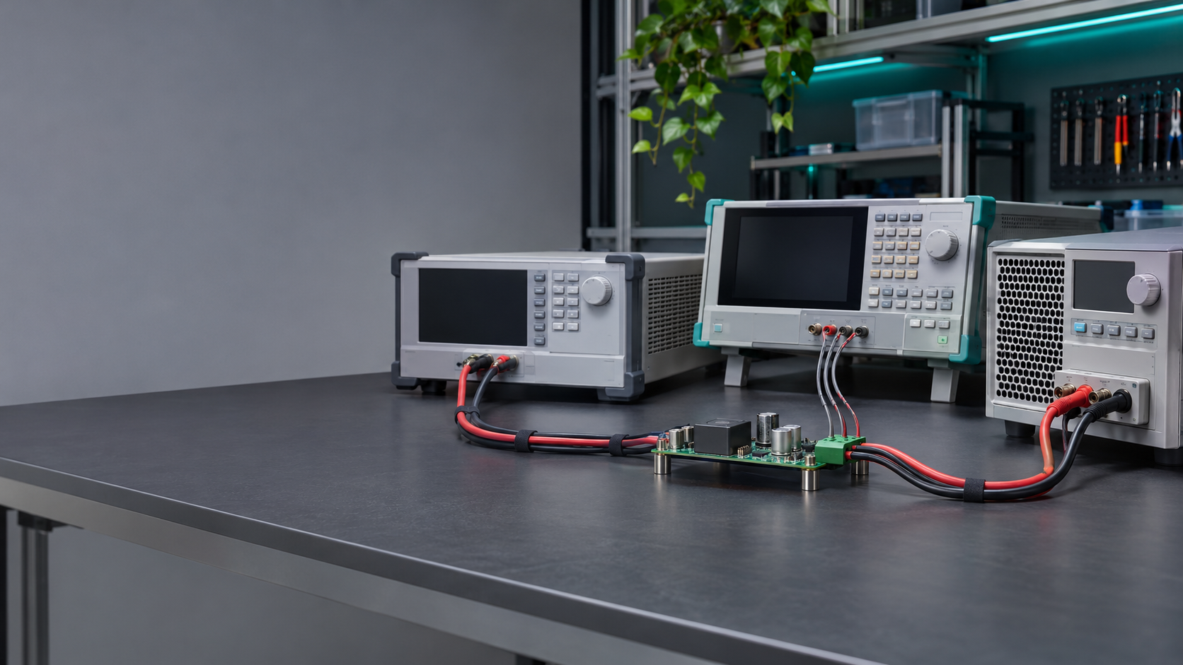
The bench setup was the simple one. Supply on a shelf, 54 V output, electronic load on a 0.6 m cable, bench DMM across the output studs, current from the load’s internal shunt, thirty minutes of soak at 25 °C. The operator put the voltmeter where the supply’s own sense leads land, which is what the datasheet implies.
The line setup was built for throughput. A fixture plate, a 1.5 m harness to a load panel, a 0.5 mΩ shunt in the return leg, sense leads at the load connector so the supply regulated at the far end. Same unit, same 14.8 A, same ambient. The number came back 1.5 points lower and the unit went to the rework bin.
Both procedures were followed. That is the part worth sitting with: a 1.5-point spread is not operator noise, it is a systematic difference between two planes, and it reproduces on every run. The unit had not changed. The ruler had.
The Path Between the Two Probes
Fifty-five milliohms is not much until you push 14.8 A through it.
| Element | Resistance | Loss at 14.8 A |
| 1.5 m of 16 AWG, out and back | 40.2 mΩ | 8.8 W |
| Two connector pairs, four contacts | 14.0 mΩ | 3.1 W |
| Current shunt and fixture wiring | 0.9 mΩ | 0.2 W |
| Total | 55.1 mΩ | 12.1 W |
Twelve watts against 800 W is 1.5%. That is the entire argument. The harness did not consume efficiency, it moved the place where efficiency was measured: the load received 12 W less than the supply produced, and the load-plane calculation put that smaller number in the numerator.
Contact resistance deserves its own line because it drifts. A crimp that measured 2 mΩ at incoming inspection can read 6 mΩ after two hundred mate cycles, and nothing in the supply’s telemetry shows it. The efficiency figure walks down across a shift and the supply gets blamed for a connector.
Sense Leads Decide the Regulation Point
Remote sensing is where this stops being arithmetic and starts changing the supply’s behavior. Keysight’s note on remote sensing sets out the mechanism: sense leads carry almost no current, so they report the voltage at their landing point, and the loop servos that node to the setpoint.
Land the sense leads on the output studs and the load sees the setpoint minus the harness drop. Land them at the load connector and the supply raises its terminal voltage until the far end reaches the setpoint. The terminals then sit about 0.8 V high, output power rises by 12 W, and input power rises to cover it. Load-plane efficiency barely moves while the supply works harder and the harness runs warmer.
That is why the record needs the sense configuration alongside the result. A unit tested with local sense and one tested with remote sense are not the same experiment at identical load current. If the record does not say which one ran, the number in it has no comparator.
Open sense leads are the other failure mode to watch. Feedback disappears, and depending on the design the output climbs until a clamp or an OVP circuit catches it. Most supplies detect an open lead or fall back to local sensing, but an intermittent sense pin produces overvoltage trips that look like a supply defect.
Regulation Is Not Efficiency
The two get conflated because both appear as percentages about the output voltage. They answer different questions. NI’s guide to line and load regulation defines them cleanly: line regulation is the voltage change for a change in input, load regulation is the change for a change in load current, and both are voltage ratios at a stated sense point.
Efficiency is a power ratio and cannot be derived from either. A supply can hold 54.00 V within ±0.05% from no load to full load and still burn 4% of its input in the converter. It can hold that voltage at the load connector while the terminals wander, because the loop is doing what remote sense asked of it.
That guide also covers cascading, which matters when two units feed one load: the pair’s efficiency is the product of the two, and the plane has to be defined once for the pair rather than per unit.
Datasheet regulation figures are comparable only when the sense point matches. Two vendors quoting ±0.1%, one at the terminals and one at the load, are not quoting the same specification.
Define the Boundary Before the Test Starts
Write the plane into the procedure and the argument disappears. Four things get fixed before the first unit is measured.
The plane itself. Output power is defined either at the supply terminals or at the load connector, and every unit in the run uses the same one. Mixing them mid-run splits a batch into pass and fail groups that do not differ electrically.
The current path. Current has to be measured in the same plane as the voltage, or V×I is not a power at any single node. A shunt upstream of the harness with a voltmeter downstream belongs to neither plane.
The sense configuration. Local or remote, lead length, wire gauge, twisted or shielded. All of it goes into the record next to the result.
The uncertainty budget. Shunt tolerance, meter accuracy on reading and range, temperature coefficients. A 0.1% shunt and a 0.05% meter combine to about 0.12% before temperature, a tenth of the effect being chased here. Small, but it has to be written down or the next disagreement has no arbiter.
The input side needs the same treatment and holds a surprising share of the error. Input power measured with a clamp and a DMM assumes sinusoidal current at unity power factor. A switching supply at light load has a displacement factor below one and a high crest factor, so VA overstates watts, sometimes by several percent. A power analyzer computing true RMS and fundamental phase is the instrument for this job.
Two smaller items belong in the same paragraph. Warm-up: thirty minutes is a convention rather than a law, but the figure drifts for the first ten. Input boundary: whether the measured input includes the auxiliary supply, the fan, and the EMI filter, since a measurement upstream of the filter is a system efficiency.
What the Line Changed Afterward
The fix was cheap and unglamorous. Sense leads moved from the supply studs to the load connector, where they belonged for a test claiming to characterize delivered power. The limit was rewritten as 94.5% at the load plane beside 96.0% at the terminals, both labeled so nobody would compare them again.
The binned unit passed on retest. Two units that had passed earlier were pulled with contact resistance above 10 mΩ in the harness, exactly the failure a terminal-plane test cannot see. The line added a harness resistance check at every shift change.
This is the boundary a production test cell has to carry explicitly rather than assume. Jettest builds power-supply test platforms around defined measurement conditions, with the instrument set and fixture depending on configuration, and the power supply application work is where those conditions get matched to what the customer’s load actually sees. The quality inspection service is where the same boundary gets audited after the fact: a procedure that does not name a plane leaves a record nobody can interpret.
What Buyers Ask at the Acceptance Review
Which plane should the acceptance number use? The one the customer’s load sees, normally the load connector. That is the node the product specification is about, and the only one that includes the harness the customer will also have. Terminal-plane data stays useful for diagnosing the supply, so keep both columns in the report and mark which one is binding.
Does remote sensing inflate the efficiency figure? It moves the loss, it does not remove it. With sense at the load the supply delivers more power at a higher terminal voltage, so input power rises and the load-plane ratio stays roughly constant. The harness dissipates the same watts either way.
How much harness drop is acceptable? Budget it as a fraction of output voltage and treat anything above your instrument uncertainty as a design input rather than a test artifact. If the drop exceeds about 1% of nominal, the harness is undersized for the current it carries.